The original jupyter notebook is on my programming_notebook repository.
Classification
Supervised learning
Unsupervised learning: Uses unlabeled data
- Uncovering hidden patterns from unlabeled data
- Example:
- Grouping customers into distinct categories (Clustering)
Reinforcement learning
- Software agents interact with an environment
- Learn how to optimize their behavior
- Given a system of rewards and punishments
- Draws inspiration from behavioral psychology
- Applications
- Economics
- Genetics
- Game playing
- AlphaGo: First computer to defeat the world champion in Go
Supervised learning
- Predictor variables/features and a target variable
- Aim: Predict the target variable, given the predictor variables
- Classification: Target variable consists of categories
- Regression: Target variable is continuous
Naming conventions
- Features = predictor variables = independent variables
- Target variable = dependent variable = response variable
Supervised learning in Python
- We will use scikit-learn/sklearn
- Integrates well with the SciPy stack
- Other libraries
- TensorFlow
- keras
Exploratory data analysis
The Iris dataset
Features:
- Petal length
- Petal width
- Sepal length
- Sepal width
Target variable: Species:
- Versicolor
- Virginica
- Setosa
The Iris dataset in scikit-learn
from sklearn import datasets
import pandas as pd
import numpy as np
import matplotlib.pyplot as plt

plt.style.use('ggplot')
iris = datasets.load_iris()
type(iris)
sklearn.utils.Bunch
print(iris.keys())
dict_keys(['data', 'target', 'target_names', 'DESCR', 'feature_names', 'filename'])
type(iris.data), type(iris.target)
(numpy.ndarray, numpy.ndarray)
iris.data.shape
(150, 4)
iris.target_names
array(['setosa', 'versicolor', 'virginica'], dtype='<U10')
Exploratory data analysis (EDA)
X = iris.data
y = iris.target
df = pd.DataFrame(X, columns=iris.feature_names)
print(df.head())
   sepal length (cm)  sepal width (cm)  petal length (cm)  petal width (cm)
0                5.1               3.5                1.4               0.2
1                4.9               3.0                1.4               0.2
2                4.7               3.2                1.3               0.2
3                4.6               3.1                1.5               0.2
4                5.0               3.6                1.4               0.2
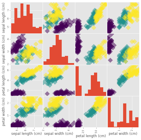
Visual EDA
_ = pd.plotting.scatter_matrix(df, c = y, figsize = [8, 8], s=150, marker = 'D')
The classification challenge
k-Nearest Neighbors
- Basic idea: Predict the label of a data point by
- Looking at the ‘k’ closest labeled data points
- Taking a majority vote
Scikit-learn fit and predict
- All machine learning models implemented as Python classes
- They implement the algorithms for learning and predicting
- Store the information learned from the data
- Training a model on the data = ‘�tting’ a model to the data
.fit()method- To predict the labels of new data:
.predict()method
Using scikit-learn to fit a classifier
from sklearn.neighbors import KNeighborsClassifier
knn = KNeighborsClassifier(n_neighbors=6)
knn.fit(iris['data'], iris['target'])
KNeighborsClassifier(algorithm='auto', leaf_size=30, metric='minkowski',
                     metric_params=None, n_jobs=None, n_neighbors=6, p=2,
                     weights='uniform')
iris['data'].shape
(150, 4)
iris['target'].shape # targets needs to be a single column with the same # of observation as the feature data
(150,)
Predicting on unlabeled data`
X_new = np.array(
[
    [5.6, 2.8, 3.9, 1.1],
    [5.7, 3.2, 3.8, 1.3],
    [4.7, 3.2, 1.3, 0.2]
])   # feature in columns and observation in rows
prediction = knn.predict(X_new)
X_new.shape # 3 obsevation and 4 colums
(3, 4)
print('Prediction: {}'.format(prediction))
Prediction: [1 1 0]
Measuring model performance
Measuring model performance
- In classification, accuracy is a commonly used metric
- Accuracy = Fraction of correct predictions
- Which data should be used to compute accuracy?
-
How well will the model perform on new data?
- Could compute accuracy on data used to fit classifier
- NOT indicative of ability to generalize
- Split data into training and test set
- Fit/train the classifier on the training set
- Make predictions on test set
- Compare predictions with the known labels
Train/test split
from sklearn.model_selection import train_test_split

# use train_test_split function to randomly split data
# firast argument is feature data, the second the targets or labels
# returns the training data, test data, training labels, test labels
# by default split the data into 75% training data and 25% test data, we specify the size using the test_size
# stratify=y:perform the split so that the split reflects the labels on your data, that is the labels to be distributed in train and test sets as they are in original dataset.
X_train, X_test, y_train, y_test = train_test_split(X, y, test_size=0.3,
    random_state=21, stratify=y)
knn = KNeighborsClassifier(n_neighbors=8)
knn.fit(X_train, y_train)
y_pred = knn.predict(X_test)

print("Test set predictions:")
print(y_pred)
Test set predictions:
[2 1 2 2 1 0 1 0 0 1 0 2 0 2 2 0 0 0 1 0 2 2 2 0 1 1 1 0 0 1 2 2 0 0 1 2 2
 1 1 2 1 1 0 2 1]
# check out accuracy of the model
knn.score(X_test, y_test)
0.9555555555555556
Model complexity
- Larger k = smoother decision boundary = less complex model
- Smaller k = more complex model = can lead to overfitting
Exercise: The digits recognition dataset
# Import necessary modules
from sklearn import datasets
import matplotlib.pyplot as plt
# Load the digits dataset: digits
digits = datasets.load_digits()
# Print the keys and DESCR of the dataset
print(digits.keys())
print(digits.DESCR)
# Print the shape of the images and data keys
print(digits.images.shape)
print(digits.data.shape)
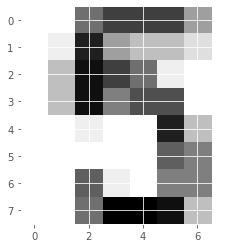
# Display the 1011th image
plt.imshow(digits.images[1010], cmap=plt.cm.gray_r, interpolation='nearest')
plt.show()
dict_keys(['data', 'target', 'target_names', 'images', 'DESCR'])
.. _digits_dataset:

Optical recognition of handwritten digits dataset
--------------------------------------------------

**Data Set Characteristics:**

    :Number of Instances: 5620
    :Number of Attributes: 64
    :Attribute Information: 8x8 image of integer pixels in the range 0..16.
    :Missing Attribute Values: None
    :Creator: E. Alpaydin (alpaydin '@' boun.edu.tr)
    :Date: July; 1998

This is a copy of the test set of the UCI ML hand-written digits datasets
https://archive.ics.uci.edu/ml/datasets/Optical+Recognition+of+Handwritten+Digits

The data set contains images of hand-written digits: 10 classes where
each class refers to a digit.

Preprocessing programs made available by NIST were used to extract
normalized bitmaps of handwritten digits from a preprinted form. From a
total of 43 people, 30 contributed to the training set and different 13
to the test set. 32x32 bitmaps are divided into nonoverlapping blocks of
4x4 and the number of on pixels are counted in each block. This generates
an input matrix of 8x8 where each element is an integer in the range
0..16. This reduces dimensionality and gives invariance to small
distortions.

For info on NIST preprocessing routines, see M. D. Garris, J. L. Blue, G.
T. Candela, D. L. Dimmick, J. Geist, P. J. Grother, S. A. Janet, and C.
L. Wilson, NIST Form-Based Handprint Recognition System, NISTIR 5469,
1994.

.. topic:: References

  - C. Kaynak (1995) Methods of Combining Multiple Classifiers and Their
    Applications to Handwritten Digit Recognition, MSc Thesis, Institute of
    Graduate Studies in Science and Engineering, Bogazici University.
  - E. Alpaydin, C. Kaynak (1998) Cascading Classifiers, Kybernetika.
  - Ken Tang and Ponnuthurai N. Suganthan and Xi Yao and A. Kai Qin.
    Linear dimensionalityreduction using relevance weighted LDA. School of
    Electrical and Electronic Engineering Nanyang Technological University.
    2005.
  - Claudio Gentile. A New Approximate Maximal Margin Classification
    Algorithm. NIPS. 2000.
(1797, 8, 8)
(1797, 64)
Train/Test Split + Fit/Predict/Accuracy
# Import necessary modules
from sklearn.neighbors import KNeighborsClassifier
from sklearn.model_selection import train_test_split

# Create feature and target arrays
X = digits.data
y = digits.target

# Split into training and test set
X_train, X_test, y_train, y_test = train_test_split(X, y, test_size = 0.2, random_state=42, stratify=y)

# Create a k-NN classifier with 7 neighbors: knn
knn = KNeighborsClassifier(n_neighbors=7)

# Fit the classifier to the training data
knn.fit(X_train, y_train)

# Print the accuracy
print(knn.score(X_test, y_test))
0.9833333333333333
Overfitting and underfitting
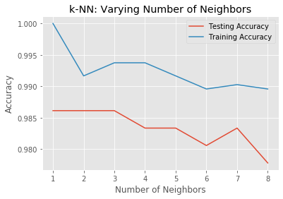
In this exercise, you will compute and plot the training and testing accuracy scores for a variety of different neighbor values. By observing how the accuracy scores differ for the training and testing sets with different values of k, you will develop your intuition for overfitting and underfitting.
# Setup arrays to store train and test accuracies
neighbors = np.arange(1, 9)
train_accuracy = np.empty(len(neighbors))
test_accuracy = np.empty(len(neighbors))

# Loop over different values of k
for i, k in enumerate(neighbors):
    # Setup a k-NN Classifier with k neighbors: knn
    knn = KNeighborsClassifier(n_neighbors=k)

    # Fit the classifier to the training data
    knn.fit(X_train, y_train)

    #Compute accuracy on the training set
    train_accuracy[i] = knn.score(X_train, y_train)

    #Compute accuracy on the testing set
    test_accuracy[i] = knn.score(X_test, y_test)

# Generate plot
plt.title('k-NN: Varying Number of Neighbors')
plt.plot(neighbors, test_accuracy, label = 'Testing Accuracy')
plt.plot(neighbors, train_accuracy, label = 'Training Accuracy')
plt.legend()
plt.xlabel('Number of Neighbors')
plt.ylabel('Accuracy')
plt.show()

# It looks like the test accuracy is highest when using 3 and 5 neighbors.
# Using 8 neighbors or more seems to result in a simple model that underfits the data.
Regression
Introduction to regression
Boston housing data
from sklearn import datasets
boston_data = datasets.load_boston()

# change to dataframe
boston = pd.DataFrame(boston_data.data, columns=boston_data.feature_names)
boston['MEDV'] = pd.Series(boston_data.target)
print(boston.head())
      CRIM    ZN  INDUS  CHAS    NOX     RM   AGE     DIS  RAD    TAX  \
0  0.00632  18.0   2.31   0.0  0.538  6.575  65.2  4.0900  1.0  296.0
1  0.02731   0.0   7.07   0.0  0.469  6.421  78.9  4.9671  2.0  242.0
2  0.02729   0.0   7.07   0.0  0.469  7.185  61.1  4.9671  2.0  242.0
3  0.03237   0.0   2.18   0.0  0.458  6.998  45.8  6.0622  3.0  222.0
4  0.06905   0.0   2.18   0.0  0.458  7.147  54.2  6.0622  3.0  222.0

   PTRATIO       B  LSTAT  MEDV
0     15.3  396.90   4.98  24.0
1     17.8  396.90   9.14  21.6
2     17.8  392.83   4.03  34.7
3     18.7  394.63   2.94  33.4
4     18.7  396.90   5.33  36.2
Creating feature and target arrays
X = boston.drop('MEDV', axis=1).values
y = boston['MEDV'].values
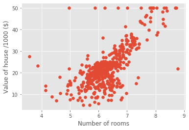
Predicting house value from a single feature
# single feature: the average num of romms in a block
X_rooms = X[:,5] # fifth column
# check type
type(X_rooms), type(y)
(numpy.ndarray, numpy.ndarray)
# Keep the first dimension, but add another dimension of size one to X,from (506,) to (506, 1)
y = y.reshape(-1, 1)
X_rooms = X_rooms.reshape(-1, 1)
X_rooms.shape
(506, 1)
Plotting house value vs. number of rooms
plt.scatter(X_rooms, y)
plt.ylabel('Value of house /1000 ($)')
plt.xlabel('Number of rooms')
plt.show();

# more rooms leads to higher prices
Fitting a regression model
import numpy as np
from sklearn.linear_model import LinearRegression
# instantiate LinearRegression as reg
reg = LinearRegression()
# fit regressor to the data
reg.fit(X_rooms, y)
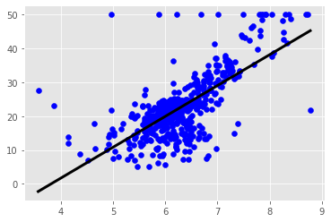
# check out the regressors predictions over the range of the data by using np.linspace between the maximum
# and minimum number of rooms and make prediction for this data
prediction_space = np.linspace(min(X_rooms),
max(X_rooms)).reshape(-1, 1)
plt.scatter(X_rooms, y, color='blue')
plt.plot(prediction_space, reg.predict(prediction_space),
    color='black', linewidth=3)
plt.show()
The basics of linear regression
Regression mechanics
- y = ax + b
- x = single feature
-
a, b = parameters of model
- How do we choose a and b?
- Define an error functions for any given line
- Choose the line that minimizes the error function
The loss function
Ordinary least squares(OLS): Minimize sum of squares of residuals
Linear regression in higher dimensions
$y = a_1x_1 +a_2x_2 + b$
- To fit a linear regression model here:
- Need to specify 3 variables
- In higher dimensions:
- Must specify coefficient for each feature and the variable b
$y = a_1x_1 +a_2x_2 + a_3x_3+ \dots +a_nx_n +b$
- Must specify coefficient for each feature and the variable b
- Scikit-learn API works exactly the same way:
- Pass two arrays: Features, and target
Linear regression on all features
from sklearn.model_selection import train_test_split
from sklearn.linear_model import LinearRegression

X_train, X_test, y_train, y_test = train_test_split(X, y, test_size = 0.3, random_state=42)
reg_all = LinearRegression()
reg_all.fit(X_train, y_train)
y_pred = reg_all.predict(X_test)
reg_all.score(X_test, y_test)
0.711226005748496
Cross-validation
Cross-validation is a vital step in evaluating a model. It maximizes the amount of data that is used to train the model, as during the course of training, the model is not only trained, but also tested on all of the available data.
Cross-validation motivation
- Model performance is dependent on way the data is split
- Not representative of the model’s ability to generalize
- Solution: Cross-validation!
Cross-validation and model performance
- Cross-validation and model performance
- 10 folds = 10-fold CV
- k folds = k-fold CV
- More folds = More computationally expensive
Cross-validation in scikit-learn
from sklearn.model_selection import cross_val_score
from sklearn.linear_model import LinearRegression

# instantiate model
reg = LinearRegression()
# call cross val score with the regressor, the feature data and the target data as the first three positional argument
# specify the numver of fold with cv
cv_results = cross_val_score(reg, X, y, cv=5)
# the length of the array is the number of folds utilized
# note that the score reported is R square(default score for linear regression)
print(cv_results)
[ 0.63919994 0.71386698 0.58702344 0.07923081 -0.25294154]
np.mean(cv_results)
0.3532759243958772
Regularized regression
Linear least squares, Lasso,ridge regression有何本质区别?
Why regularize?
- Recall: Linear regression minimizes a loss function
- It chooses a coefficient for each feature variable
- Large coefficients can lead to overfitting
- Penalizing large coefficients: Regularization
Ridge regression
- Loss function = OLS loss function + $\alpha * \sum_{i=1}^n \alpha_i^2$
- Alpha: Parameter we need to choose
- Picking alpha here is similar to picking k in k-NN
- Hyperparameter tuning (More in Chapter 3)
- Alpha controls model complexity
- Alpha = 0: We get back OLS (Can lead to overfitting)
- Very high alpha: Can lead to underfitting
from sklearn.linear_model import Ridge

X_train, X_test, y_train, y_test = train_test_split(X, y, test_size = 0.3, random_state=42)
# set up alpha, normalize insure all the variables are on the same scale
ridge = Ridge(alpha=0.1, normalize=True)
ridge.fit(X_train, y_train)
ridge_pred = ridge.predict(X_test)
ridge.score(X_test, y_test)
0.6996938275127313
Lasso regression
-
Loss function = OLS loss function + $\alpha * \sum_{i=1}^n \alpha_i $
from sklearn.linear_model import Lasso

X_train, X_test, y_train, y_test = train_test_split(X, y,
    test_size = 0.3, random_state=42)
lasso = Lasso(alpha=0.1, normalize=True)
# Fit the regressor to the data
lasso.fit(X_train, y_train)
lasso_pred = lasso.predict(X_test)
lasso.score(X_test, y_test)
0.5950229535328551
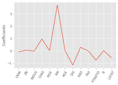
Lasso regression for feature selection
- Can be used to select important features of a dataset
- Shrinks the coefficients of less important features to exactly 0
from sklearn.linear_model import Lasso
names = boston.drop('MEDV', axis=1).columns
lasso = Lasso(alpha=0.1)
# Compute and print the coefficients,extract the coef attribute and store in lasso coef
lasso_coef = lasso.fit(X, y).coef_
# plotting the coefficients as a function of feature name
_ = plt.plot(range(len(names)), lasso_coef)
_ = plt.xticks(range(len(names)), names, rotation=60)
_ = plt.ylabel('Coefficients')
plt.show()
# Lasso selected out the 'RM' feature as being the most important for predicting
# Boston house prices, while shrinking the coefficients of certain other features to 0.
Fine-tuning your model
How good is your model?
Classification metrics
- Measuring model performance with accuracy:
- Fraction of correctly classified samples
- Not always a useful metric
Class imbalance example: Emails
- Spam classification
- 99% of emails are real; 1% of emails are spam
- Could build a classifier that predicts ALL emails as real
- 99% accurate!
- But horrible at actually classifying spam
- Fails at its original purpose
- Need more nuanced metrics
Diagnosing classification predictions
- Confusion matrix
| Predicted: Spam Email | Predicted: Real Email | |
|---|---|---|
| Actual: Spam Email | True Positive | False Negative |
| Actual: Real Email | False Positive | True Negative |
Metrics from the confusion matrix
-
Accuracy:$\frac{tp+tn}{tp+tn+fp+fn}$
-
Precision:$\frac{tp}{tp+fp}$
-
Recall: $\frac{tp}{tp+fn}$
-
F1score: $2* \frac{Precision* Recall}{Precisio+Recall}$
-
High precision: Not many real emails predicted as spam
-
High recall: Predicted most spam emails correctly
iris = datasets.load_iris()
X = iris.data
y = iris.target
df = pd.DataFrame(X, columns=iris.feature_names)

# Import necessary modules
from sklearn.metrics import classification_report
from sklearn.metrics import confusion_matrix

# Instantiate a k-NN classifier: knn
knn = KNeighborsClassifier(n_neighbors=8)
# Create training and test set
X_train, X_test, y_train, y_test = train_test_split(X, y,
    test_size=0.4, random_state=42)
# Fit the classifier to the training data
knn.fit(X_train, y_train)
# Predict the labels of the test data: y_pred
y_pred = knn.predict(X_test)
# compute confusion matrix
print(confusion_matrix(y_test, y_pred))
[[23  0  0]
 [ 0 19  0]
 [ 0  1 17]]
# compute result matrix
print(classification_report(y_test, y_pred))
              precision    recall  f1-score   support

           0       1.00      1.00      1.00        23
           1       0.95      1.00      0.97        19
           2       1.00      0.94      0.97        18

    accuracy                           0.98        60
   macro avg       0.98      0.98      0.98        60
weighted avg       0.98      0.98      0.98        60
Logistic regression and the ROC curve
Logistic regression for binary classification
- Logistic regression outputs probabilities
- If the probability ‘p’ is greater than 0.5:
- The data is labeled ‘1’
- If the probability ‘p’ is less than 0.5:
- The data is labeled ‘0’
from sklearn.linear_model import LogisticRegression
from sklearn.model_selection import train_test_split

import warnings
warnings.filterwarnings("ignore", category=FutureWarning)

logreg = LogisticRegression()
X_train, X_test, y_train, y_test = train_test_split(X, y, test_size=0.4, random_state=42)
logreg.fit(X_train, y_train)
y_pred = logreg.predict(X_test)
Probability thresholds
- By default, logistic regression threshold = 0.5
- Not specific to logistic regression
- k-NN classifiers also have thresholds
- What happens if we vary the threshold?
Exercise
Building a logistic regression model
Time to build your first logistic regression model! scikit-learn makes it very easy to try different models, since the Train-Test-Split/Instantiate/Fit/Predict paradigm applies to all classifiers and regressors - which are known in scikit-learn as ‘estimators’. You’ll see this now for yourself as you train a logistic regression model on exactly the same data as in the previous exercise. Will it outperform k-NN? There’s only one way to find out!
diabetes = pd.read_csv("data/diabetes.csv")

X = diabetes.drop('diabetes', axis=1).values
y = diabetes['diabetes'].values
# Import the necessary modules
from sklearn.linear_model import LogisticRegression
from sklearn.metrics import confusion_matrix, classification_report

# Create training and test sets
X_train, X_test, y_train, y_test = train_test_split(X, y, test_size = 0.4, random_state=42)

# Create the classifier: logreg
logreg = LogisticRegression()

# Fit the classifier to the training data
logreg.fit(X_train, y_train)

# Predict the labels of the test set: y_pred
y_pred = logreg.predict(X_test)

# Compute and print the confusion matrix and classification report
print(confusion_matrix(y_test, y_pred))
print(classification_report(y_test, y_pred))
[[174  32]
 [ 36  66]]
              precision    recall  f1-score   support

           0       0.83      0.84      0.84       206
           1       0.67      0.65      0.66       102

    accuracy                           0.78       308
   macro avg       0.75      0.75      0.75       308
weighted avg       0.78      0.78      0.78       308
Plotting an ROC curve
Classification reports and confusion matrices are great methods to quantitatively evaluate model performance, while ROC curves provide a way to visually evaluate models. As Hugo demonstrated in the video, most classifiers in scikit-learn have a .predict_proba() method which returns the probability of a given sample being in a particular class. Having built a logistic regression model, you’ll now evaluate its performance by plotting an ROC curve. In doing so, you’ll make use of the .predict_proba() method and become familiar with its functionality.
Here, you’ll continue working with the PIMA Indians diabetes dataset. The classifier has already been fit to the training data and is available as logreg.
# Import necessary modules
from sklearn.metrics import roc_curve

# Compute predicted probabilities: y_pred_prob
y_pred_prob = logreg.predict_proba(X_test)[:,1]

# Generate ROC curve values: fpr, tpr, thresholds
fpr, tpr, thresholds = roc_curve(y_test, y_pred_prob)

# Plot ROC curve
plt.plot([0, 1], [0, 1], 'k--')
plt.plot(fpr, tpr)
plt.xlabel('False Positive Rate')
plt.ylabel('True Positive Rate')
plt.title('ROC Curve')
plt.show()
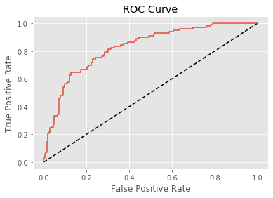
Area under the ROC curve
- Larger area under the ROC curve(AUC) = better model
Exercise
AUC computation
Say you have a binary classifier that in fact is just randomly making guesses. It would be correct approximately 50% of the time, and the resulting ROC curve would be a diagonal line in which the True Positive Rate and False Positive Rate are always equal. The Area under this ROC curve would be 0.5. This is one way in which the AUC, is an informative metric to evaluate a model. If the AUC is greater than 0.5, the model is better than random guessing. Always a good sign!
In this exercise, you’ll calculate AUC scores using the roc_auc_score() function from sklearn.metrics as well as by performing cross-validation on the diabetes dataset.
# Import necessary modules
from sklearn.metrics import roc_auc_score
from sklearn.model_selection import cross_val_score

# Compute predicted probabilities: y_pred_prob
y_pred_prob = logreg.predict_proba(X_test)[:,1]

# Compute and print AUC score
print("AUC: {}".format(roc_auc_score(y_test, y_pred_prob)))

# Compute cross-validated AUC scores: cv_auc
cv_auc = cross_val_score(logreg, X, y, cv=5, scoring='roc_auc')

# Print list of AUC scores
print("AUC scores computed using 5-fold cross-validation: {}".format(cv_auc))
AUC: 0.8268608414239482
AUC scores computed using 5-fold cross-validation: [0.7987037  0.80777778 0.81944444 0.86622642 0.85037736]
Hyperparameter tuning
- Linear regression: Choosing parameters
- Ridge/lasso regression: Choosing alpha
- k-Nearest Neighbors: Choosing n_neighbors Parameters like alpha and k: Hyperparameters
- Hyperparameters cannot be learned by fitting the model
Choosing the correct hyperparameter
- Try a bunch of different hyperparameter values Fit all of them separately
- See how well each performs
- Choose the best performing one
- It is essential to use cross-validation
GridSearchCV in scikit-learn
from sklearn.model_selection import GridSearchCV
# specify the hyperparameter as a dictionary in which the keys are the dictionary
# which the keys are the hyperparameter names, such as n_neighbors in KNN or alpha in lasso regression.
# The values in the grid dictionary are lists containing the values we wish to tune the relevant hyperparameter(s) over
# if specify multiple parameters, all possible combinations will be tried
param_grid = {'n_neighbors': np.arange(1, 50)}
# ibnstantiate classifier
knn = KNeighborsClassifier()
# pass our model(knn), the gird we wish to tune over(param_grid) and the # of folds that we wish to use
knn_cv = GridSearchCV(knn, param_grid, cv=5) # return a GridSearch object that can fit the data
# This fit performs the actual grid search inplace
knn_cv.fit(X, y)
# apply the attributes beat params, to show the hyperparameter perform the best
knn_cv.best_params_
{'n_neighbors': 14}
# apply the attributes beat score(mean cross validation score over that fold)
knn_cv.best_score_
0.7578125
Exercise
Hyperparameter tuning with GridSearchCV
Hugo demonstrated how to tune the n_neighbors parameter of the KNeighborsClassifier() using GridSearchCV on the voting dataset. You will now practice this yourself, but by using logistic regression on the diabetes dataset instead!
Like the alpha parameter of lasso and ridge regularization that you saw earlier, logistic regression also has a regularization parameter: C. C controls the inverse of the regularization strength, and this is what you will tune in this exercise. A large C can lead to an overfit model, while a small C can lead to an underfit model.
The hyperparameter space for C has been setup for you. Your job is to use GridSearchCV and logistic regression to find the optimal C in this hyperparameter space. The feature array is available as X and target variable array is available as y.
# Import necessary modules
from sklearn.linear_model import LogisticRegression
from sklearn.model_selection import GridSearchCV

# Setup the hyperparameter grid by using c_space as the grid of values to tune C over.
c_space = np.logspace(-5, 8, 15)
param_grid = {'C': c_space }

# Instantiate a logistic regression classifier: logreg
logreg = LogisticRegression()

# Instantiate the GridSearchCV object: logreg_cv
logreg_cv = GridSearchCV(logreg, param_grid, cv=5) # specify the classifier, parameter grid, and number of folds to use.

# Fit it to the data
logreg_cv.fit(X, y)

# Print the tuned parameters and score
print("Tuned Logistic Regression Parameters: {}".format(logreg_cv.best_params_))
print("Best score is {}".format(logreg_cv.best_score_))
Tuned Logistic Regression Parameters: {'C': 268.2695795279727}
Best score is 0.7708333333333334
Hyperparameter tuning with RandomizedSearchCV
GridSearchCV can be computationally expensive, especially if you are searching over a large hyperparameter space and dealing with multiple hyperparameters. A solution to this is to use RandomizedSearchCV, in which not all hyperparameter values are tried out. Instead, a fixed number of hyperparameter settings is sampled from specified probability distributions. You’ll practice using RandomizedSearchCV in this exercise and see how this works.
Here, you’ll also be introduced to a new model: the Decision Tree. Don’t worry about the specifics of how this model works. Just like k-NN, linear regression, and logistic regression, decision trees in scikit-learn have .fit() and .predict() methods that you can use in exactly the same way as before. Decision trees have many parameters that can be tuned, such as max_features, max_depth, and min_samples_leaf: This makes it an ideal use case for RandomizedSearchCV.
# Import necessary modules
from scipy.stats import randint
from sklearn.tree import DecisionTreeClassifier
from sklearn.model_selection import RandomizedSearchCV

# Setup the parameters and distributions to sample from: param_dist
param_dist = {"max_depth": [3, None],
              "max_features": randint(1, 9),
              "min_samples_leaf": randint(1, 9),
              "criterion": ["gini", "entropy"]}

# Instantiate a Decision Tree classifier: tree
tree = DecisionTreeClassifier()

# Instantiate the RandomizedSearchCV object: tree_cv
tree_cv = RandomizedSearchCV(tree, param_dist, cv=5)

# Fit it to the data
tree_cv.fit(X, y)
RandomizedSearchCV(cv=5, error_score='raise-deprecating',
                   estimator=DecisionTreeClassifier(class_weight=None,
                                                    criterion='gini',
                                                    max_depth=None,
                                                    max_features=None,
                                                    max_leaf_nodes=None,
                                                    min_impurity_decrease=0.0,
                                                    min_impurity_split=None,
                                                    min_samples_leaf=1,
                                                    min_samples_split=2,
                                                    min_weight_fraction_leaf=0.0,
                                                    presort=False,
                                                    random_state=None,
                                                    splitter='best'),
                   iid='w...None,
                   param_distributions={'criterion': ['gini', 'entropy'],
                                        'max_depth': [3, None],
                                        'max_features': <scipy.stats._distn_infrastructure.rv_frozen object at 0x7f8a0b827710>,
                                        'min_samples_leaf': <scipy.stats._distn_infrastructure.rv_frozen object at 0x7f8a0ccc1f10>},
                   pre_dispatch='2*n_jobs', random_state=None, refit=True,
                   return_train_score=False, scoring=None, verbose=0)
Note that RandomizedSearchCV will never outperform GridSearchCV. Instead, it is valuable because it saves on computation time.
Hold-out set for final evaluation
Hold-out set reasoning
- How well can the model perform on never before seen data?
- Using ALL data for cross-validation is not ideal
- Split data into training and hold-out set at the beginning
- Perform grid search cross-validation on training set
- Choose best hyperparameters and evaluate on hold-out set
Exercise
Hold-out set in practice I: Classification
You will now practice evaluating a model with tuned hyperparameters on a hold-out set. The feature array and target variable array from the diabetes dataset have been pre-loaded as X and y.
In addition to C, logistic regression has a 'penalty' hyperparameter which specifies whether to use 'l1' or 'l2' regularization. Your job in this exercise is to create a hold-out set, tune the 'C' and 'penalty' hyperparameters of a logistic regression classifier using GridSearchCV on the training set.
diabetes = pd.read_csv("data/diabetes.csv")

X = diabetes.drop('diabetes', axis=1)

y = diabetes['diabetes']
# handle missing data
# instaniate an instance of the imputer
from sklearn.preprocessing import Imputer
imp = Imputer(missing_values=0, strategy='mean', axis=0) # axis=0, impute along columns
imp.fit(X)
X = imp.transform(X) # due to their ability to transform our data as such, impters are known as transformers
X
array([[  6.   , 148.   ,  72.   , ...,  33.6  ,   0.627,  50.   ],
       [  1.   ,  85.   ,  66.   , ...,  26.6  ,   0.351,  31.   ],
       [  8.   , 183.   ,  64.   , ...,  23.3  ,   0.672,  32.   ],
       ...,
       [  5.   , 121.   ,  72.   , ...,  26.2  ,   0.245,  30.   ],
       [  1.   , 126.   ,  60.   , ...,  30.1  ,   0.349,  47.   ],
       [  1.   ,  93.   ,  70.   , ...,  30.4  ,   0.315,  23.   ]])
# Import necessary modules
from sklearn.model_selection import train_test_split
from sklearn.linear_model import LogisticRegression
from sklearn.model_selection import GridSearchCV

import warnings
warnings.filterwarnings(action='ignore',category=DeprecationWarning)

# Create the hyperparameter grid
c_space = np.logspace(-5, 8, 15)
param_grid = {'C': c_space, 'penalty': ['l1', 'l2']}

# Instantiate the logistic regression classifier: logreg
logreg = LogisticRegression()

# Create train and test sets
X_train, X_test, y_train, y_test = train_test_split(X, y, test_size = 0.4, random_state=42)

# Instantiate the GridSearchCV object: logreg_cv
logreg_cv = GridSearchCV(logreg, param_grid, cv=5)

# Fit it to the training data
logreg_cv.fit(X_train, y_train)

# Print the optimal parameters and best score
print("Tuned Logistic Regression Parameter: {}".format(logreg_cv.best_params_))
print("Tuned Logistic Regression Accuracy: {}".format(logreg_cv.best_score_))
Tuned Logistic Regression Parameter: {'C': 3.727593720314938, 'penalty': 'l1'}
Tuned Logistic Regression Accuracy: 0.7695652173913043
Hold-out set in practice II: Regression
Remember lasso and ridge regression from the previous chapter? Lasso used the L1 penalty to regularize, while ridge used the L2 penalty. There is another type of regularized regression known as the elastic net. In elastic net regularization, the penalty term is a linear combination of the L1 and L2 penalties:
$a∗L1+b∗L2$
In scikit-learn, this term is represented by the 'l1_ratio' parameter: An 'l1_ratio' of 1 corresponds to an L1 penalty, and anything lower is a combination of L1 and L2.
In this exercise, you will GridSearchCV to tune the 'l1_ratio' of an elastic net model trained on the Gapminder data. As in the previous exercise, use a hold-out set to evaluate your model’s performance.
# Import necessary modules
from sklearn.linear_model import ElasticNet
from sklearn.metrics import mean_squared_error
from sklearn.model_selection import GridSearchCV
from sklearn.model_selection import train_test_split

# Create train and test sets
X_train, X_test, y_train, y_test = train_test_split(X, y, test_size=0.4, random_state=42)

# Create the hyperparameter grid
l1_space = np.linspace(0, 1, 30)
param_grid = {'l1_ratio': l1_space}

# Instantiate the ElasticNet regressor: elastic_net
elastic_net = ElasticNet()

# Setup the GridSearchCV object: gm_cv
gm_cv = GridSearchCV(elastic_net, param_grid, cv=5)

# Fit it to the training data
gm_cv.fit(X_train, y_train)

# Predict on the test set and compute metrics
y_pred = gm_cv.predict(X_test)
r2 = gm_cv.score(X_test, y_test)
mse = mean_squared_error(y_test, y_pred)
print("Tuned ElasticNet l1 ratio: {}".format(gm_cv.best_params_))
print("Tuned ElasticNet R squared: {}".format(r2))
print("Tuned ElasticNet MSE: {}".format(mse))
Tuned ElasticNet l1 ratio: {'l1_ratio': 0.13793103448275862}
Tuned ElasticNet R squared: 0.2508917697155366
Tuned ElasticNet MSE: 0.16592450386592536
Preprocessing and pipelines
Preprocessing data
Dealing with categorical features
- Scikit-learn will not accept categorical features by default
- Need to encode categorical features numerically
- Convert to ‘dummy variables’
- 0: Observation was NOT that category
- 1: Observation was that category
Dealing with categorical features in Python
- scikit-learn: OneHotEncoder()
- pandas: get_dummies()
Automobile dataset
- mpg: Target Variable
- Origin: Categorical Feature
Encoding dummy variables
 import pandas as pd
df = pd.read_csv('data/auto.csv')
df_origin = pd.get_dummies(df)
print(df_origin.head())
    mpg  displ   hp  weight  accel  size  origin_Asia  origin_Europe  \
0  18.0  250.0   88    3139   14.5  15.0            0              0
1   9.0  304.0  193    4732   18.5  20.0            0              0
2  36.1   91.0   60    1800   16.4  10.0            1              0
3  18.5  250.0   98    3525   19.0  15.0            0              0
4  34.3   97.0   78    2188   15.8  10.0            0              1

   origin_US
0          1
1          1
2          0
3          1
4          0
df_origin = df_origin.drop('origin_Asia', axis=1)
print(df_origin.head())
    mpg  displ   hp  weight  accel  size  origin_Europe  origin_US
0  18.0  250.0   88    3139   14.5  15.0              0          1
1   9.0  304.0  193    4732   18.5  20.0              0          1
2  36.1   91.0   60    1800   16.4  10.0              0          0
3  18.5  250.0   98    3525   19.0  15.0              0          1
4  34.3   97.0   78    2188   15.8  10.0              1          0
Linear regression with dummy variables
X = boston.drop('MEDV', axis=1).values
y = boston['MEDV'].values
from sklearn.model_selection import train_test_split
from sklearn.linear_model import Ridge

X_train, X_test, y_train, y_test = train_test_split(X, y, test_size=0.3, random_state=42)
ridge = Ridge(alpha=0.5, normalize=True).fit(X_train, y_train)
ridge.score(X_test, y_test)
0.6658827571518846
Exercise
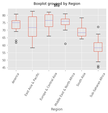
Exploring categorical features
The Gapminder dataset that you worked with in previous chapters also contained a categorical 'Region' feature, which we dropped in previous exercises since you did not have the tools to deal with it. Now however, you do, so we have added it back in!
Your job in this exercise is to explore this feature. Boxplots are particularly useful for visualizing categorical features such as this.
# Import pandas
import pandas as pd

# Read 'gapminder.csv' into a DataFrame: df
df = pd.read_csv('data/gapminder.csv')

# Create a boxplot of life expectancy per region
df.boxplot('life', 'Region', rot=60)

# Show the plot
plt.show()
Creating dummy variables
As Andy discussed in the video, scikit-learn does not accept non-numerical features. You saw in the previous exercise that the 'Region' feature contains very useful information that can predict life expectancy. For example, Sub-Saharan Africa has a lower life expectancy compared to Europe and Central Asia. Therefore, if you are trying to predict life expectancy, it would be preferable to retain the 'Region' feature. To do this, you need to binarize it by creating dummy variables, which is what you will do in this exercise.
# Create dummy variables: df_region
df_region = pd.get_dummies(df)

# Print the columns of df_region
print(df_region.columns)

# Create dummy variables with drop_first=True: df_region
df_region = df_region.drop('Region_America', axis=1)
# or: df_region = pd.get_dummies(df, drop_first=True)

# Print the new columns of df_region
print(df_region.columns)
Index(['population', 'fertility', 'HIV', 'CO2', 'BMI_male', 'GDP',
       'BMI_female', 'life', 'child_mortality', 'Region_America',
       'Region_East Asia & Pacific', 'Region_Europe & Central Asia',
       'Region_Middle East & North Africa', 'Region_South Asia',
       'Region_Sub-Saharan Africa'],
      dtype='object')
Index(['population', 'fertility', 'HIV', 'CO2', 'BMI_male', 'GDP',
       'BMI_female', 'life', 'child_mortality', 'Region_East Asia & Pacific',
       'Region_Europe & Central Asia', 'Region_Middle East & North Africa',
       'Region_South Asia', 'Region_Sub-Saharan Africa'],
      dtype='object')
Regression with categorical features
Having created the dummy variables from the 'Region' feature, you can build regression models as you did before. Here, you’ll use ridge regression to perform 5-fold cross-validation.
The feature array X and target variable array y have been pre-loaded.
# Import necessary modules
from sklearn.model_selection import cross_val_score
from sklearn.linear_model import Ridge

# Instantiate a ridge regressor: ridge
ridge = Ridge(alpha=0.5, normalize=True)

# Perform 5-fold cross-validation: ridge_cv
ridge_cv = cross_val_score(ridge, X, y, cv=5)

# Print the cross-validated scores
print(ridge_cv)
[0.66758848 0.69340446 0.47352712 0.24855188 0.29564884]
Handling missing data
PIMA Indians dataset
df = pd.read_csv('data/diabetes.csv')
df.info()
<class 'pandas.core.frame.DataFrame'>
RangeIndex: 768 entries, 0 to 767
Data columns (total 9 columns):
pregnancies    768 non-null int64
glucose        768 non-null int64
diastolic      768 non-null int64
triceps        768 non-null int64
insulin        768 non-null int64
bmi            768 non-null float64
dpf            768 non-null float64
age            768 non-null int64
diabetes       768 non-null int64
dtypes: float64(2), int64(7)
memory usage: 54.1 KB
print(df.head())
   pregnancies  glucose  diastolic  triceps  insulin   bmi    dpf  age  \
0            6      148         72       35        0  33.6  0.627   50
1            1       85         66       29        0  26.6  0.351   31
2            8      183         64        0        0  23.3  0.672   32
3            1       89         66       23       94  28.1  0.167   21
4            0      137         40       35      168  43.1  2.288   33

   diabetes
0         1
1         0
2         1
3         0
4         1
Dropping missing data
df.insulin.replace(0, np.nan, inplace=True)
df.triceps.replace(0, np.nan, inplace=True)
df.bmi.replace(0, np.nan, inplace=True)
df.info()
<class 'pandas.core.frame.DataFrame'>
RangeIndex: 768 entries, 0 to 767
Data columns (total 9 columns):
pregnancies    768 non-null int64
glucose        768 non-null int64
diastolic      768 non-null int64
triceps        541 non-null float64
insulin        394 non-null float64
bmi            757 non-null float64
dpf            768 non-null float64
age            768 non-null int64
diabetes       768 non-null int64
dtypes: float64(4), int64(5)
memory usage: 54.1 KB
df = df.dropna() # remove columns contain Nan
df.shape # half of rows droped, unacceptable
(393, 9)
Imputing missing data
- Making an educated guess about the missing values
- Example: Using the mean of the non-missing entries
# instaniate an instance of the imputer
from sklearn.preprocessing import Imputer
imp = Imputer(missing_values='NaN', strategy='mean', axis=0) # axis=0, impute along columns
imp.fit(X)
X = imp.transform(X) # due to their ability to transform our data as such, impters are known as transformers
Imputing within a pipeline
- Making an educated guess about the missing values
- Example: Using the mean of the non-missing entries
from sklearn.pipeline import Pipeline
from sklearn.preprocessing import Imputer

imp = Imputer(missing_values='NaN', strategy='mean', axis=0)
logreg = LogisticRegression()
# construct a list of steps in the pipeline, where each step is a 2-tuple containing the name you wish to give the relevant step and the estimator
steps = [('imputation', imp), ('logistic_regression', logreg)]
# pass the list to the pipeline constructor
pipeline = Pipeline(steps)
X_train, X_test, y_train, y_test = train_test_split(X, y, test_size=0.3, random_state=42)
pipeline.fit(X_train, y_train.astype('int'))
y_pred = pipeline.predict(X_test)
# compute acurracy
pipeline.score(X_test, y_test.astype('int'))
0.06578947368421052
Note: in a pipeline, each step but the last must be a transformer and the last must be an estimator, such as, a classifier or a regressor
Exercise
Dropping missing data
The voting dataset from Chapter 1 contained a bunch of missing values that we dealt with for you behind the scenes. Now, it’s time for you to take care of these yourself!
The unprocessed dataset has been loaded into a DataFrame df. Explore it in the IPython Shell with the .head() method. You will see that there are certain data points labeled with a ‘?'. These denote missing values. As you saw in the video, different datasets encode missing values in different ways. Sometimes it may be a '9999', other times a 0 - real-world data can be very messy! If you’re lucky, the missing values will already be encoded as NaN. We use NaN because it is an efficient and simplified way of internally representing missing data, and it lets us take advantage of pandas methods such as .dropna() and .fillna(), as well as scikit-learn’s Imputation transformer Imputer().
In this exercise, your job is to convert the '?'s to NaNs, and then drop the rows that contain them from the DataFrame.
df = voting

# Convert '?' to NaN
df[df == '?'] = np.nan

# Print the number of NaNs
print(df.isnull().sum())

# Print shape of original DataFrame
print("Shape of Original DataFrame: {}".format(df.shape))

# Drop missing values and print shape of new DataFrame
df = df.dropna()

# Print shape of new DataFrame
print("Shape of DataFrame After Dropping All Rows with Missing Values: {}".format(df.shape))
party                  0
infants               12
water                 48
budget                11
physician             11
salvador              15
religious             11
satellite             14
aid                   15
missile               22
immigration            7
synfuels              21
education             31
superfund             25
crime                 17
duty_free_exports     28
eaa_rsa              104
dtype: int64
Shape of Original DataFrame: (435, 17)
Shape of DataFrame After Dropping All Rows with Missing Values: (232, 17)
When many values in your dataset are missing, if you drop them, you may end up throwing away valuable information along with the missing data. It’s better instead to develop an imputation strategy. This is where domain knowledge is useful, but in the absence of it, you can impute missing values with the mean or the median of the row or column that the missing value is in.
Imputing missing data in a ML Pipeline I
As you’ve come to appreciate, there are many steps to building a model, from creating training and test sets, to fitting a classifier or regressor, to tuning its parameters, to evaluating its performance on new data. Imputation can be seen as the first step of this machine learning process, the entirety of which can be viewed within the context of a pipeline. Scikit-learn provides a pipeline constructor that allows you to piece together these steps into one process and thereby simplify your workflow.
You’ll now practice setting up a pipeline with two steps: the imputation step, followed by the instantiation of a classifier. You’ve seen three classifiers in this course so far: k-NN, logistic regression, and the decision tree. You will now be introduced to a fourth one - the Support Vector Machine, or SVM. For now, do not worry about how it works under the hood. It works exactly as you would expect of the scikit-learn estimators that you have worked with previously, in that it has the same .fit() and .predict() methods as before.
df = voting
df[df == 'y'] = 1
df[df == 'n'] = 0
df[df == '?'] = "NaN"
# Import the Imputer module
from sklearn.svm import SVC
from sklearn.preprocessing import Imputer

# Setup the Imputation transformer: imp
imp = Imputer(missing_values='NaN', strategy='most_frequent', axis=0)

# Instantiate the SVC classifier: clf
clf = SVC()

# Setup the pipeline with the required steps: steps
steps = [('imputation', imp),
        ('SVM', clf)]
Imputing missing data in a ML Pipeline II
Having setup the steps of the pipeline in the previous exercise, you will now use it on the voting dataset to classify a Congressman’s party affiliation. What makes pipelines so incredibly useful is the simple interface that they provide. You can use the .fit() and .predict() methods on pipelines just as you did with your classifiers and regressors!
Practice this for yourself now and generate a classification report of your predictions. The steps of the pipeline have been set up for you, and the feature array X and target variable array y have been pre-loaded. Additionally, train_test_split and classification_report have been imported from sklearn.model_selection and sklearn.metrics respectively.
X = df.drop('party', axis=1)
y = df['party']
# Import necessary modules
from sklearn.preprocessing import Imputer
from sklearn.pipeline import Pipeline
from sklearn.svm import SVC

# Setup the pipeline steps: steps
steps = [('imputation', Imputer(missing_values='NaN', strategy='most_frequent', axis=0)),
        ('SVM', SVC())]

# Create the pipeline: pipeline
pipeline = Pipeline(steps)

# Create training and test sets
X_train, X_test, y_train, y_test = train_test_split(X, y, test_size=0.3, random_state=42)

# Fit the pipeline to the train set
pipeline.fit(X_train, y_train)

# Predict the labels of the test set
y_pred = pipeline.predict(X_test)

# Compute metrics
print(classification_report(y_test, y_pred))
              precision    recall  f1-score   support

    democrat       0.99      0.96      0.98        85
  republican       0.94      0.98      0.96        46

    accuracy                           0.97       131
   macro avg       0.96      0.97      0.97       131
weighted avg       0.97      0.97      0.97       131
Centering and scaling
Why scale your data?
- Many models use some form of distance to inform them
- Features on larger scales can unduly infiuence the model
- Example: k-NN uses distance explicitly when making predictions
- We want features to be on a similar scale
- Normalizing (or scaling and centering)
Ways to normalize your data
- Standardization: Subtract the mean and divide by variance
- All features are centered around zero and have variance one
- Can also subtract the minimum and divide by the range Minimum zero and maximum one
- Can also normalize so the data ranges from -1 to +1
- See scikit-learn docs for further details
Scaling in scikit-learn
winequality_red = pd.read_csv("data/winequality-red.csv")
winequality_red
| fixed acidity | volatile acidity | citric acid | residual sugar | chlorides | free sulfur dioxide | total sulfur dioxide | density | pH | sulphates | alcohol | quality | |
|---|---|---|---|---|---|---|---|---|---|---|---|---|
| 0 | 7.4 | 0.700 | 0.00 | 1.9 | 0.076 | 11.0 | 34.0 | 0.99780 | 3.51 | 0.56 | 9.4 | 5 |
| 1 | 7.8 | 0.880 | 0.00 | 2.6 | 0.098 | 25.0 | 67.0 | 0.99680 | 3.20 | 0.68 | 9.8 | 5 |
| 2 | 7.8 | 0.760 | 0.04 | 2.3 | 0.092 | 15.0 | 54.0 | 0.99700 | 3.26 | 0.65 | 9.8 | 5 |
| 3 | 11.2 | 0.280 | 0.56 | 1.9 | 0.075 | 17.0 | 60.0 | 0.99800 | 3.16 | 0.58 | 9.8 | 6 |
| 4 | 7.4 | 0.700 | 0.00 | 1.9 | 0.076 | 11.0 | 34.0 | 0.99780 | 3.51 | 0.56 | 9.4 | 5 |
| ... | ... | ... | ... | ... | ... | ... | ... | ... | ... | ... | ... | ... |
| 1594 | 6.2 | 0.600 | 0.08 | 2.0 | 0.090 | 32.0 | 44.0 | 0.99490 | 3.45 | 0.58 | 10.5 | 5 |
| 1595 | 5.9 | 0.550 | 0.10 | 2.2 | 0.062 | 39.0 | 51.0 | 0.99512 | 3.52 | 0.76 | 11.2 | 6 |
| 1596 | 6.3 | 0.510 | 0.13 | 2.3 | 0.076 | 29.0 | 40.0 | 0.99574 | 3.42 | 0.75 | 11.0 | 6 |
| 1597 | 5.9 | 0.645 | 0.12 | 2.0 | 0.075 | 32.0 | 44.0 | 0.99547 | 3.57 | 0.71 | 10.2 | 5 |
| 1598 | 6.0 | 0.310 | 0.47 | 3.6 | 0.067 | 18.0 | 42.0 | 0.99549 | 3.39 | 0.66 | 11.0 | 6 |
1599 rows × 12 columns
print(winequality_red.describe())
       fixed acidity  volatile acidity  citric acid  residual sugar  \
count    1599.000000       1599.000000  1599.000000     1599.000000
mean        8.319637          0.527821     0.270976        2.538806
std         1.741096          0.179060     0.194801        1.409928
min         4.600000          0.120000     0.000000        0.900000
25%         7.100000          0.390000     0.090000        1.900000
50%         7.900000          0.520000     0.260000        2.200000
75%         9.200000          0.640000     0.420000        2.600000
max        15.900000          1.580000     1.000000       15.500000

         chlorides  free sulfur dioxide  total sulfur dioxide      density  \
count  1599.000000          1599.000000           1599.000000  1599.000000
mean      0.087467            15.874922             46.467792     0.996747
std       0.047065            10.460157             32.895324     0.001887
min       0.012000             1.000000              6.000000     0.990070
25%       0.070000             7.000000             22.000000     0.995600
50%       0.079000            14.000000             38.000000     0.996750
75%       0.090000            21.000000             62.000000     0.997835
max       0.611000            72.000000            289.000000     1.003690

                pH    sulphates      alcohol      quality
count  1599.000000  1599.000000  1599.000000  1599.000000
mean      3.311113     0.658149    10.422983     5.636023
std       0.154386     0.169507     1.065668     0.807569
min       2.740000     0.330000     8.400000     3.000000
25%       3.210000     0.550000     9.500000     5.000000
50%       3.310000     0.620000    10.200000     6.000000
75%       3.400000     0.730000    11.100000     6.000000
max       4.010000     2.000000    14.900000     8.000000
X = winequality_red.drop('quality', axis=1).values
y = winequality_red['quality'].values
y = np.where(y<5, 1, 0)
from sklearn.preprocessing import scale
X_scaled = scale(X)
np.mean(X), np.std(X)
(8.134219224515322, 16.726533979432848)
np.mean(X_scaled), np.std(X_scaled)
(2.546626531486538e-15, 1.0)
Scaling in a pipeline
from sklearn.preprocessing import StandardScaler
steps = [('scaler', StandardScaler()),('knn', KNeighborsClassifier())]
pipeline = Pipeline(steps)
# split dartaset in training and test set
X_train, X_test, y_train, y_test = train_test_split(X, y, test_size=0.2, random_state=21)
# fit the pipeline to training set
knn_scaled = pipeline.fit(X_train, y_train)
# predict test set
y_pred = pipeline.predict(X_test)
# compute accuracy
accuracy_score(y_test, y_pred) # 0.956
# perform KNN without scaling
knn_unscaled = KNeighborsClassifier().fit(X_train, y_train)
knn_unscaled.score(X_test, y_test) # result accurancy of 0.928, scaling did improve our model performance
0.946875
CV and scaling in a pipeline
# build pipeline
steps = [('scaler', StandardScaler()), (('knn', KNeighborsClassifier()))]
pipeline = Pipeline(steps)
# specify yhperparameter space by creating a dictionary: the keys are pipeline step name followed by a double underscore,
# followed by the hyperparameter name, the corresponding vale is a list or an array of the values to try for that
# particular hyperparameter. In this case, we are tuning only the n neighbours in the KNN model
parameters = {knn__n_neighbors: np.arange(1, 50)}
# split data into cross-validation and hold-out set
X_train, X_test, y_train, y_test = train_test_split(X, y, test_size=0.2, random_state=21)
# perform gridsearch over the parameters in the pipeline by instantiating the GridSearchCV object
cv = GridSearchCV(pipeline, param_grid=parameters)
# fit to training data
cv.fit(X_train, y_train)
# The predict method will call predict on the estimator with the best found parameters and we do this on the hold-out set
y_pred = cv.predict(X_test)
Scaling and CV in a pipeline
print(cv.best_params_) # {'knn__n_neighbors': 41}
print(cv.score(X_test, y_test) )# 0.956
print(classification_report(y_test, y_pred))
Exercise
Centering and scaling your data
In the video, Hugo demonstrated how significantly the performance of a model can improve if the features are scaled. Note that this is not always the case: In the Congressional voting records dataset, for example, all of the features are binary. In such a situation, scaling will have minimal impact.
You will now explore scaling for yourself on a new dataset - White Wine Quality! Hugo used the Red Wine Quality dataset in the video. We have used the 'quality' feature of the wine to create a binary target variable: If 'quality' is less than 5, the target variable is 1, and otherwise, it is 0.
The DataFrame has been pre-loaded as df, along with the feature and target variable arrays X and y. Explore it in the IPython Shell. Notice how some features seem to have different units of measurement. 'density', for instance, takes values between 0.98 and 1.04, while 'total sulfur dioxide' ranges from 9 to 440. As a result, it may be worth scaling the features here. Your job in this exercise is to scale the features and compute the mean and standard deviation of the unscaled features compared to the scaled features.
winequality_white = pd.read_csv("data/winequality-white.csv")

X = winequality_white.drop('quality', axis=1).values
y = winequality_white['quality'].values
y = np.where(y<5, 0, 1)
# Import scale
from sklearn.preprocessing import scale

# Scale the features: X_scaled
X_scaled = scale(X)

# Print the mean and standard deviation of the unscaled features
print("Mean of Unscaled Features: {}".format(np.mean(X)))
print("Standard Deviation of Unscaled Features: {}".format(np.std(X)))

# Print the mean and standard deviation of the scaled features
print("Mean of Scaled Features: {}".format(np.mean(X_scaled)))
print("Standard Deviation of Scaled Features: {}".format(np.std(X_scaled)))
Mean of Unscaled Features: 18.432687072460002
Standard Deviation of Unscaled Features: 41.54494764094571
Mean of Scaled Features: 2.739937614267761e-15
Standard Deviation of Scaled Features: 0.9999999999999999
Centering and scaling in a pipeline
With regard to whether or not scaling is effective, the proof is in the pudding! See for yourself whether or not scaling the features of the White Wine Quality dataset has any impact on its performance. You will use a k-NN classifier as part of a pipeline that includes scaling, and for the purposes of comparison, a k-NN classifier trained on the unscaled data has been provided.
The feature array and target variable array have been pre-loaded as X and y. Additionally, KNeighborsClassifier and train_test_split have been imported from sklearn.neighbors and sklearn.model_selection, respectively.
# Import the necessary modules
from sklearn.preprocessing import StandardScaler
from sklearn.pipeline import Pipeline

# Setup the pipeline steps: steps
steps = [('scaler', StandardScaler()),
        ('knn', KNeighborsClassifier())]

# Create the pipeline: pipeline
pipeline = Pipeline(steps)

# Create train and test sets
X_train, X_test, y_train, y_test = train_test_split(X, y, test_size=0.3, random_state=42)

# Fit the pipeline to the training set: knn_scaled
knn_scaled = pipeline.fit(X_train, y_train)

# Instantiate and fit a k-NN classifier to the unscaled data
knn_unscaled = KNeighborsClassifier().fit(X_train, y_train)

# Compute and print metrics
print('Accuracy with Scaling: {}'.format(knn_scaled.score(X_test, y_test)))
print('Accuracy without Scaling: {}'.format(knn_unscaled.score(X_test, y_test)))
Accuracy with Scaling: 0.964625850340136
Accuracy without Scaling: 0.9666666666666667
It looks like scaling has improved model performance!
Bringing it all together I: Pipeline for classification
It is time now to piece together everything you have learned so far into a pipeline for classification! Your job in this exercise is to build a pipeline that includes scaling and hyperparameter tuning to classify wine quality.
You’ll return to using the SVM classifier you were briefly introduced to earlier in this chapter. The hyperparameters you will tune are C and gamma. C controls the regularization strength. It is analogous to the C you tuned for logistic regression in Chapter 3, while gamma controls the kernel coefficient: Do not worry about this now as it is beyond the scope of this course.
# Setup the pipeline
steps = [('scaler', StandardScaler()),
         ('SVM', SVC())]

pipeline = Pipeline(steps)

# Specify the hyperparameter space
# Specify the hyperparameter space using the following notation: 'step_name__parameter_name'.
# Here, the step_name is SVM, and the parameter_names are C and gamma.
parameters = {'SVM__C':[1, 10, 100],
              'SVM__gamma':[0.1, 0.01]}

# Create train and test sets
X_train, X_test, y_train, y_test = train_test_split(X, y, test_size=0.2, random_state=21)

# Instantiate the GridSearchCV object: cv
cv = GridSearchCV(pipeline, param_grid=parameters)

# Fit to the training set
cv.fit(X_train, y_train)

# Predict the labels of the test set: y_pred
y_pred = cv.predict(X_test)

# Compute and print metrics
print("Accuracy: {}".format(cv.score(X_test, y_test)))
print(classification_report(y_test, y_pred))
print("Tuned Model Parameters: {}".format(cv.best_params_))
Accuracy: 0.9693877551020408
              precision    recall  f1-score   support

           0       0.43      0.10      0.17        29
           1       0.97      1.00      0.98       951

    accuracy                           0.97       980
   macro avg       0.70      0.55      0.58       980
weighted avg       0.96      0.97      0.96       980

Tuned Model Parameters: {'SVM__C': 100, 'SVM__gamma': 0.01}
Bringing it all together II: Pipeline for regression
For this final exercise, you will return to the Gapminder dataset. Guess what? Even this dataset has missing values that we dealt with for you in earlier chapters! Now, you have all the tools to take care of them yourself!
Your job is to build a pipeline that imputes the missing data, scales the features, and fits an ElasticNet to the Gapminder data. You will then tune the l1_ratio of your ElasticNet using GridSearchCV.
All the necessary modules have been imported, and the feature and target variable arrays have been pre-loaded as X and y.
# Setup the pipeline steps: steps
steps = [('imputation', Imputer(missing_values='NaN', strategy='mean', axis=0)),
         ('scaler', StandardScaler()),
         ('elasticnet', ElasticNet())]

# Create the pipeline: pipeline
pipeline = Pipeline(steps)

# Specify the hyperparameter space
# Specify the hyperparameter space for the l1 ratio using the following notation:
# 'step_name__parameter_name'. Here, the step_name is elasticnet, and the parameter_name is l1_ratio.
parameters = {'elasticnet__l1_ratio':np.linspace(0,1,30)}

# Create train and test sets
X_train, X_test, y_train, y_test = train_test_split(X, y, test_size=0.4, random_state=42)

# Create the GridSearchCV object: gm_cv
gm_cv = GridSearchCV(pipeline, param_grid=parameters)

# Fit to the training set
gm_cv.fit(X_train, y_train)

# Compute and print the metrics
r2 = gm_cv.score(X_test, y_test)
print("Tuned ElasticNet Alpha: {}".format(gm_cv.best_params_))
print("Tuned ElasticNet R squared: {}".format(r2))
Tuned ElasticNet Alpha: {'elasticnet__l1_ratio': 0.0}
Tuned ElasticNet R squared: 0.03467831194788973